Freight Network Design | Francisco Zenteno Smith

This is a personal project inspired by professor and friend Armin Lüer https://scholar.google.com/citations?user=9F69pKwAAAAJ.

Repository here: https://github.com/fjzs/turkey_network

1 Introduction

1.1 What is a hub location problem?

Hubs location problems fall within the broad category of network design problems, where a private or public firm has the task of producing/moving and/or delivering its products efficiently to its customer through some facilities. In particular, a hub is a type of facility used to consolidate the flow from multiple sources to leverage economies of scale in the transportation. These are used in multiple situations, such as in passenger transportation (both in land and air), cargo , postal mail delivery (before e-mail was invented though), public services , and more.

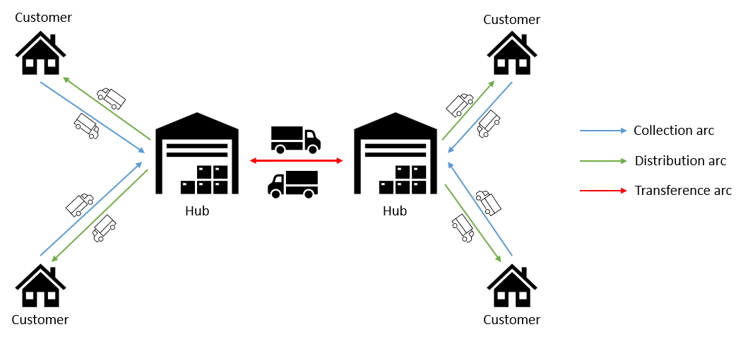
In this project there are 3 types of arcs where different logistic activities occur: collection, transference and distribution, which you can see in the next figure. I am going to assume that small trucks are used for collection and distribution activities, and that big and faster trucks are used for transference activities.

This hub location problem contains 3 types of arcs. Collection is related to the delivery of cargo from origin nodes to hubs. Transference is related to the movement of cargo between hubs. Distribution is related to the delivery of cargo from hubs to destination hubs. In the transference arc is where the economy of scale is achieved, both in speed and cost by a fixed factor.

1.2 Characteristics of our problem

A freight cargo company wants to enter to the Turkey cargo market, providing service to all the 81 provinces in the country. We assume there are other companies in the market, and so to compete properly, this new company will provide a guaranteed time delivery service for all origin-destination pairs. To do this it will localize some hubs, assign cities to hubs and determine which hubs are going to be connected to each other. The demand is given by all pairs of origin-destination cities, and the proposed network has to comply with:

Cargo must be transported through hubs, in other words, it is not allowed to transport directly between nodes that are not hubs.
There is no capacity constraints in the hubs or in the arcs.
Each origin-destination flow must pass through at least 1 and maximum 2 hubs.
Each customer must be assigned to a single hub for simplicity of management.
The latest arrival time to from every origin to every destination has to be at most $\beta$ hours.
Every hub, before transporting cargo to other hubs, must wait for all its assignated customers to bring their cargo to consolidate. In other words, the departuring time of a hub when going to other hub is equivalent to the latest arrival of cargo from its assignated customers.
Every hub, before delivering cargo to its customers, must wait for all incoming cargo from other hubs to consolidate. In other words, the departuring time of a hub when going to its customers is equivalent to the latest arrival of cargo from other hubs.
There is no time needed to consolidate cargo.
The demand is fixed and inelastic to the service level offered.
For simplicity, I will assume that only the top $k=20$ largest provinces are available to locate hubs.

The costs to consider are:

Fixed cost of locating a hub in a particular province.
Fixed cost of establishing a connection between 2 hubs or between a province and a hub.
Cost of transporting cargo on each arc of the network (collection, transfer and distribution) per unit of distance.
Economy of scale factor $\alpha$ of using large and specialized trucks between hubs (for instance 10% cheaper and 10% faster).

Turkey is an interesting case of study because:

There are no clear simmetries in the demand (north v/s south, or east v/s west)
There are big nodes of supply/demand distributed across the country (the biggest node, for instance, is Istanbul located in the northwest)
The country has a reasonable infrastructure for land transportation, allowing the possibility of every province to be connected to the network.

In the following picture you can see the 81 provinces of Turkey.

I discretized this continous representation into a set of nodes, all connected to each other by the highways of the country. Each node representing the province is located at the major city of that province. In the following diagram you can see the discretized representation of the country:

This illustration shows the borders of Turkey along with its 81 major provinces. The size of each node is proportional to the population of that province. Source: own work

1.3 Where does the data come from?

The distances between each pair of provinces was taken from Tan and Kara (2007), although Google Maps could have been used as well.
The economy of scale factor $\alpha$ was taken by a survey from Tan and Kara (2007), where they interviewed major freight companies in Turkey. The value is roughly 0.9 (although they only used it for discounting the transportation cost, and I am going to use it to decrease the speed of trucks as well)
The flow between each pair of provinces is given by Çetiner et al. (2007), which is proportional to the population of both provinces
The fixed cost for stablishing a link between hubs was taken by Alumur et al (2009), which is proportional to the distance and inversely proportional to the flow between them.
The fixed cost of stablishing a hub was taken from Alumur et al (2009).

1.4 Questions to answer

The purpose of this project is to answer these questions:

What is the optimal network design and cost structure given a time delivery service $\beta$?
How does that solution change as $\beta$ changes?
How does that solution change as the economy of scale factor $\alpha$ changes?

2 Optimization Model

The optimization model I designed is the fusion between Tan and Kara (2006) “A Hub Covering Model for Cargo Delivery Systems” and Ernst and Krishnamoorthy (1996) “Efficient algorithms for the uncapacitated single allocation p-Hub median problem”. It is also related to Alumur et al (2009) “The design of single allocation incomplete hub networks”.

Tan and Kara (2006) take care of the delivery time modelling without transportation and fixed costs.
Ernst and Krishnamoorthy (1996) take care of the network modelling without service levels.

I modelled the problem as a multicommodity flow problem, where each origin is a commodity. Just as in Alumur et al (2009), this model has $O(n^2)$ binary variables and $O(n^3)$ continuous variables, but I don’t fix the number of hubs to locate or the number of links to stablish a priori as Alumur et al (2009) did.

2.1 Sets

$N$: set of nodes

2.2 Parameters

$w_{ij}$: flow from node $i$ to node $j$ (boxes)

$s_i = \sum_{j \in N}w_{ij}$: supply of node $i$ (boxes)

$h_i$: fixed cost of locating a hub at node $i$ ($)

$d_{ij}$: distance between nodes $i$ and $j$ (km)

$v$: velocity of trucks (km/h)

$t_{ij} = d_{ij} / v$: travel time by regular (in collection and distribution activities) truck between nodes $i$ and $j$ (h)

$f_{ij}$: fixed cost of using arc $(i,j)$ ($)

$c$: unit cost of transporting 1 box 1 km ($/box-km)

$\alpha$: economy of scale factor in transfer activities between hubs (unitless)

$\beta$: maximum time delivery between any origin and destination (h)

2.3 Variables

$Z_{ik}$: 1 if node $i$ is assigned to hub $k$ else 0, $\forall i \in N, k \in N$ (unitless)

$F_{ik}$: flow from node $i$ to hub $k$, $\forall i \in N, k \in N$ (boxes)

$Y_{ikl}$: flow from node $i$ going through hubs $k$ and $l$, $\forall i \in N, k \in N, l \in K: k \neq l, i \neq l$ (boxes)

$X_{ilj}$: flow from node $i$ going through hub $l$ to destination $j$, $\forall i \in N, l \in N, j \in N: i \neq j$ (boxes)

$R_{kl}$: 1 if hub $k$ is connected to hub $l$ else 0, $\forall k \in N, l \in N: k \neq l$ (unitless)

$D^{h}_k$: departure time from hub $k$ to transport cargo to other hubs, $\forall k \in N$ (h)

$D^{c}_k$: departure time from hub $k$ to transport cargo to customers, $\forall k \in N$ (h)

$A_j$: latest arrival time to destination $j$, $\forall j \in N$ (h)

2.4 Objective Function

Location hubs cost:

\[\sum_{i \in N} Z_{ii} \cdot h_i\]

Links between nodes cost:

\[\sum_{i \in N}\sum_{k \in N} Z_{ik} \cdot f_{ik} + \sum_{k \in N}\sum_{l \in N} R_{kl} \cdot f_{kl}\]

Transportation cost (collection activities):

\[\sum_{i \in N}\sum_{k \in N} F_{ik} \cdot d_{ik} \cdot c\]

Transportation cost (transfer activities):

\[\sum_{i \in N}\sum_{k \in N}\sum_{l \in N} Y_{ikl} \cdot d_{kl}\cdot c \cdot \alpha\]

Transportation cost (distribution activities):

\[\sum_{i \in N}\sum_{l \in N}\sum_{j \in N} X_{ilj} \cdot d_{lj}\cdot c\]

2.5 Constraints

(1) Assign every node to a single hub:

\[\sum_{k \in N}Z_{ik}= 1\] \[\forall i \in N\]

(2) Assigning a node to a hub implies the hub is located:

\[Z_{ik} \leq Z_{kk}\] \[\forall i \in N, k \in N: i \neq k\]

(3) The flow from each node goes fully to it’s hub:

\[F_{ik} = Z_{ik} \cdot s_i\] \[\forall i \in N, k \in N\]

(4) Flow from origin between hubs implies link between them:

\[Y_{ikl} \leq R_{kl} \cdot s_i\] \[\forall i \in N, k \in N, l \in N: k \neq l, i \neq l\]

(5) Conservation of flow from origin $i$ at hub $k$:

\[F_{ik} + \sum_{h \in N}Y_{ihk} = \sum_{l \in N}Y_{ikl} + \sum_{j \in N}X_{ikj}\] \[\forall i \in N, k \in N\]

(6) Flow from origin between hubs implies origin assigned to hub:

\[Y_{ikl} \leq Z_{ik} \cdot s_i\] \[\forall i \in N, k \in N, l \in N: k \neq l, l \neq i\]

(7) Flow from origin to destination covered:

\[X_{ilj} = Z_{jl} \cdot w_{ij}\] \[\forall i \in N, l \in N, j \in N: i \neq j\]

(8) Link between hubs implies hubs:

\[2R_{kl} \leq Z_{kk} + Z_{ll}\] \[\forall k \in N, l \in N: k \neq l\]

(9) Truck departuring from hub $k$ to other hubs must wait for cargo from customers:

\[D^{h}_k \geq t_{ik} \cdot Z_{ik}\] \[\forall i \in N, k \in N: i \neq k\]

(10) Truck departure time from hub $l$ to its customers must wait for incoming cargo from other hubs:

Original non-linear:

\[D^{c}_l \geq (D^{h}_k + t_{kl} \cdot \alpha) \cdot R_{kl}\]

When linearized:

\[D^{c}_{l} \geq D^{h}_k + t_{kl} \cdot \alpha - M(1 - R_{kl})\]

Where $M$ is a large enough number, in this case $M = \beta$.

\[\forall k \in N, l \in N\]

(11) Truck departure time from hub $l$ to its customer $j$ must wait from all customers to consolidate cargo (this is required for the case when a single hub is located to the network).

\[D^{c}_{l} \geq t_{jl} \cdot Z_{jl}\] \[\forall j \in N, l \in N\]

(12) Latest arrival to customer $j$ depends on the latest truck arriving to its assigned hub $l$:

Original non-linear:

\[A_j \geq (D^{c}_{l} + t_{lj}) \cdot Z_{jl}\]

When linearized:

\[A_j \geq D^{c}_{l} + t_{lj} - M(1 - Z{jl})\]

Where $M$ is a large enough number, in this case $M = \beta$.

\[\forall j \in N, l \in N\]

(13) Latest arrival to destination $j$ satisfies the service level:

\[A_j \leq \beta\] \[\forall j \in N\]

2.6 Toy example to visualize variables relations

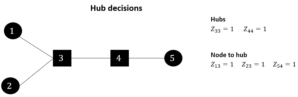
Let’s look at a little example of 5 nodes to understand visually how they interact. We will take a look at 3 types of variables: hub decisions, flow decisions and timing decisions. In the figure below we start with the hub decisions.

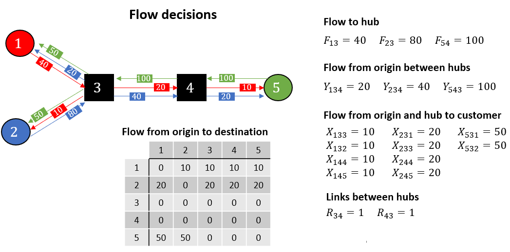
In this diagram you can see the network was organized with 2 hubs (nodes 3 and 4).

Now we can move forward with flow decisions. Remember the flow is modeled as a multi-commodity problem, where each origin is a commodity. In the figure below you can see how the flow from each origin moves through the network.

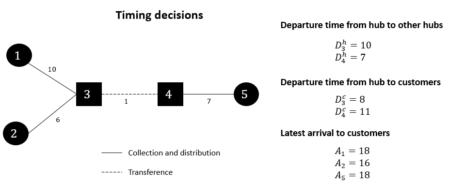
In this diagram you can see how each origin (I painted with red, blue and green the nodes the supply flow to the network) transports its flow. Recall that this is an uncapacitated problem, so there are no capacity constraints in the arcs of the graph.

Finally we can see the timing decisions in the next figure. From this example we can conclude that the latest delivery service level time is 18 time units.

In this diagram you can see how the timings are organized. Recall that the freight between non-hub nodes and hubs is supposed to be done in regular trucks, and the freight between hubs in cheaper and faster trucks. The number on each arc represent the time needed to traverse it.

3 Implementation

In this section I’ll take about the software side of this project and the hardware that I used to run it.

3.1 Software

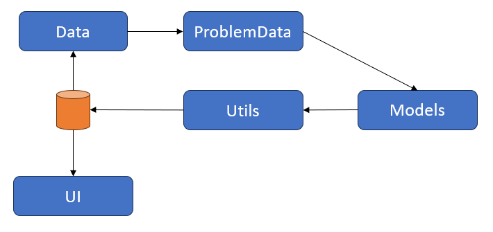
The following Figure shows a simplified view of system architecture.

Data: is the module responsible for reading the files containing the information of this problem.
ProblemData: exposes an API for the Models module, encapsulating all the data needed for this optimization problem.
Models: this module has 1 or more optimization models that uses the ProblemData API to solve the problem. Currently it is coupled with Gurobi.
Utils: this module is responsible for saving a solution into a file and to load it as well into memory.
UI: this module is responsible for reading a solution from a file and presenting it to the user.

System architecture: each blue element is a module or package in the application. The black arrows represent how the information flows through them and which modules are connected to each other.

3.2 Hardware

I ran all the experiments in my personal laptop:

OS: Windows 11
Processor: 12th Gen Intel Core i5 12 Cores
RAM: 16 Gb

4 Results

The first question to answer is: how does the solution change as $\beta$ changes? To do this I set up 3 values for $\beta=30,34,40$ hours and solved to optimality all these instances. In the next figure you will see the optimal network for each value, and in the next one you will see the optimal cost structure for reach solution.

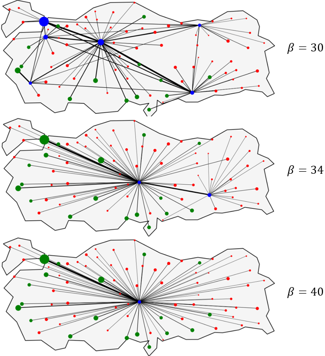
This figure shows the optimal network structure for each value of beta, the service level (max time delivery between each pair of origin and destination provinces). The size of each node is proportional to its population. Blue nodes represent hubs, green and red dots represent non-hubs, and green dots are potential hubs location that were not chosen as hubs by the model.

On each color you can see the cost component in the objective function

Couple of points from these 2 figures:

The model is solving for all the 81 provinces in Turkey
Current parameter of economy of scale factor is $\alpha=0.8$
The best service level achievable is $\beta=30$, and the network required 6 hubs, all connected to each other to satisfy this requirement.
At $\beta=40$ there is no need for economies of scale, the service level constraint is not activated. But as we start to increase it, of course, the need for economies of scale (in speed) is required with an increase in cost of roughly 20%.
This analysis could be useful for a company when evaluating the cost required to provide a service level in the network. For instance, it is rougly twice as expensive to provide a service level of $\beta=30$ v/s $\beta=40$. And the current operational structure does not allow for this service level to be faster.

The second question to answer is: how does the solution change as $\alpha$ changes? In other words, what is the economic and operational effect of improving the current technology in hub-to-hub trucks when maintaining the service level $(\beta=30)$? Just as before, I set up 3 values for $\alpha=0.6, 0.7, 0.8$ and solved to optimality. In the next 2 figures you will see the optimal network and cost structure for each instance.

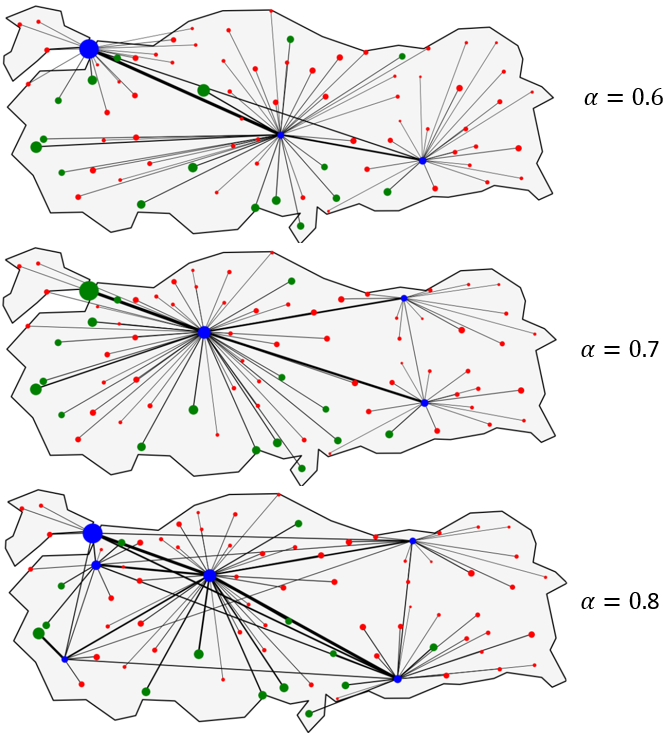
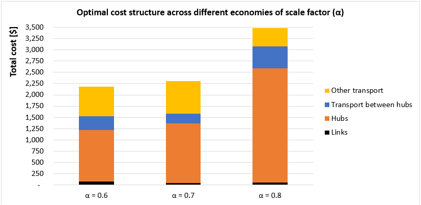
This figure shows the optimal network structure for each value of alpha, the economy of scale factor (how faster and cheaper is the transportation between hubs). The size of each node is proportional to its population. Blue nodes represent hubs, green and red dots represent non-hubs, and green dots are potential hubs location that were not chosen as hubs by the model.

Couple of points from these 2 figures:

The case where $\alpha=0.8$ is the same network as in the previous example with $\beta=30$, in other words, this is our base case.
Notice how the network simplifies (number of hubs and links between them) as $\alpha$ decreases.
The major reduction in cost is given when going from $\alpha=0.8$ to $\alpha=0.7$, which implies a cost reduction from $3,500 to $2,250 (35%). This is because the number of hubs required decreased (which was the major component of the cost).
This analysis could be useful for a company when evaluating the impact of a new technology providing faster or cheaper transport when consolidating cargo.

5 Extensions

This problem exhibits several dimensions to be extended, for instance:

Faster solution methods: because we have $O(n^2)$ binary variables and $O(n^3)$ continuous variables, a descomposition approach such as Benders could be applied here.
More complex operational design: capacity constraints could be added, elasticity in the demand and different service levels among pairs of origin-destination
Dynamic models instead of static: the decision of localizing a facility is a strategic decision which should be evaluated in financial terms for a long term horizon. This could be added as well, with a demand forecast and with the financial characteristic for this company. Also, the fixed costs in a dynamic model could weight less because of the potential gains in operational expenses in the future.