Designing a mini Roomba | Francisco Zenteno Smith

This project is part of the course “Introduction to Robotics” taught by professor Henrik Christensen in the Computer Science Department at UC San Diego. Link of the course is here: http://www.hichristensen.net/CSE276A-23/index.html

Project repository: https://github.com/fjzs/mobile-robotics-2d

1 Problem Definition

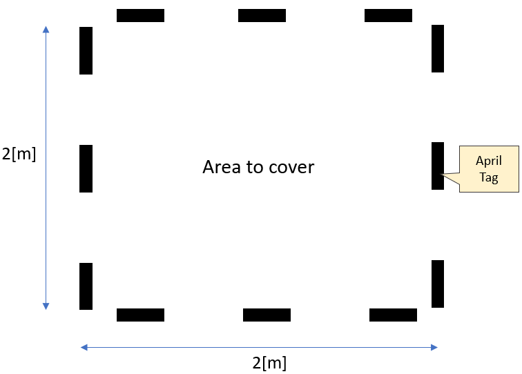
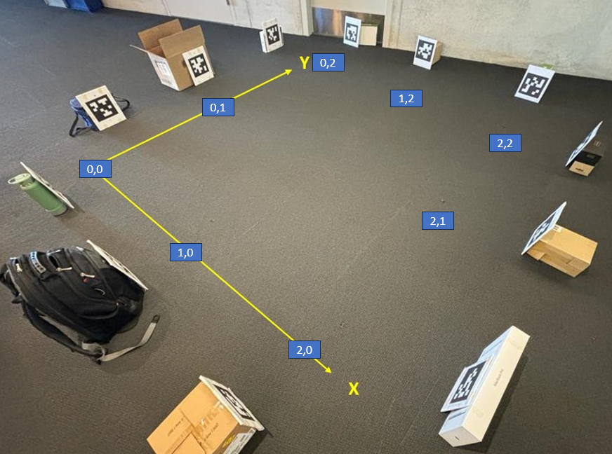
Given a Four Mecanum Wheeled Mobile Robot, design a “Roomba”-like system for a 2 x 2 square meters zone (free of obstacles). Use 12 April Tags to localize the robot as shown in Figure 1. Provide an algorithm to clean the zone, a video of it and a performance guarantee for this coverage.

Figure 1: the area to cover is a square 2x2 square meters surrounded by april tags to help localize the robot.

1.1 What is a Four Mecanum Wheeled Mobile Robot?

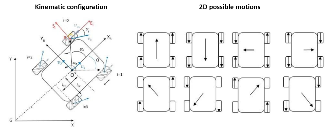
A mecanum wheel is an omnidirectional wheel design, providing the capability to move in 2D and rotate along the z axis, as opposed to traditional wheels that can only move in 1D. In this project we followed and implemented the kinematic model provided by Taheri et al (2015) (https://research.ijcaonline.org/volume113/number3/pxc3901586.pdf). In Figure 2 you can see the kinematic configuration of this robot. Each wheel \(i\) has an angular velocity of \(\omega_i\), providing the robot with a 2D velocity \((v_x, v_y)\) and a rotation around the z axis (yaw) given by \(\omega_z\).

Figure 2: On the left you can see the kinematic configuration of this robot. Notice that the robot coordinate frame is located at the center of the robot (O), and Xr axis is towards the front of the robot, and Yr is towards the left of the robot. Source: Taheri et al (2015)

1.2 The particular robot used

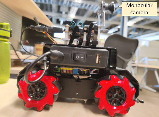
In this project the robot consisted in a Mbot Mega (4 mecanum wheel robot) + Qualcomm RB5 board. This robot is equipped with a monocular camera that we will use for perceptions tasks. You can see it in Figure 3.

Figure 3: this is the robot we used, which provides enough computing resources and a camera to perform multiple robotic tasks.

1.3 What is an April Tag and how to use it for localization

April Tag is a visual system developed at University of Michigan (https://april.eecs.umich.edu/software/apriltag). It’s like a QR code that can be read by a library developed by the authors. In Figure 4 there is a description of how this works. Given the coordinate frames of the world (w), robot (r), robot’s camera (c) and april tag (a), when the robot’s camera reads an april tag, the library retrieves both the id of the tag and the 4x4 transformation \(^{c}T_{a}\), which is the relative transformation that takes a point in the april tag coordinate frame to the robot’s camera coordinate frame. Then, using that \(^{c}T_{a} = (^{a}T_{c})^{-1}\), we can get the robot position (x,y,z) and orientation (roll, pitch, yaw) in the world frame using the following equation:

\[^{w}T_{r} = ^{w}T_{a} \cdot ^{a}T_{c} \cdot ^{c}T_{r}\]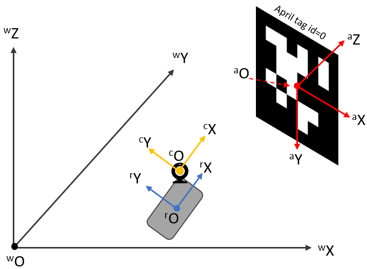

Figure 4: An april tag is like a QR code that when read by the April Tag library, returns the id of the tag and the relative position and orientation of the camera with respect to the april tag. In this diagram we have 4 coordinate frames: the world frame (w), the robot frame (r), the robot's camera frame (c) and the april tag frame (a). Here we show the april tag id=0 for family 36h11 specifically, but there are multiple families and ids of april tags.

2 Solution

We used ROS + python as the main framework to develop this project. The environment of this project is shown in Figure 5.

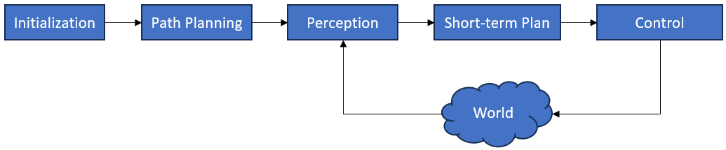
Figure 5: This is a 2x2 meters zone that the robot must cover. We have 12 april tags at fixed positions and orientations that will provide localization to the robot.

The architecture of our system is shown in Figure 6. In the next subsections we explain the responsibilities of each module.

2.1 Initialization

This module is responsible for configuring the environment and the robot in the system, such as:

The size of the environment
The coordinate frame of the world frame
The transformations matrices (orientation and position) of each april tag in world frame
The initial position of the robot
The transformations matrices of the robot’s camera with respect to the robot
The time interval of the loop (for instance, 0.05 seconds)
The parameters of the kinematic model of the robot

2.2 Path Planning

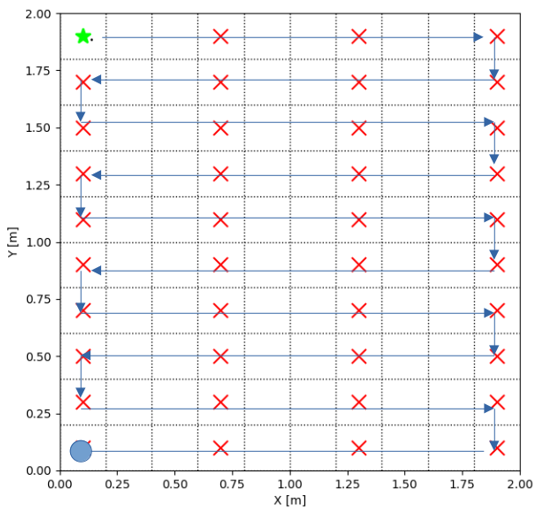
This module is responsible for providing a set of waypoints \((x, y, \theta)\) for the robot to follow in order to cover the area. To do this, first a world representation is created, which in this case corresponds to a 2D grid. The size of each cell is a parameter of the module. In this project we chose to use 0.2 [m] as the cell side length, because the robot length is roughly 0.2 [m] as well. Then, given this grid, another algorithm decides how to cover it. In this case we chose a mine sweeper style to cover the grid (graph), which is shown in Figure 7.

Figure 7: the robot starts in the green start and goes through the waypoints (red Xs) all the way down to the blue circle. We decided to spread the waypoints in this fashion because of the noise of the sensors.

2.3 Perception

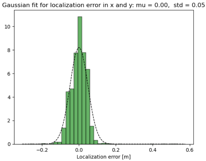
The only sensor of this robot is the camera, which is used to detect April Tags. Then, as shown in section 1.3, we can use the April Tag library to estimate the robot state given by its position and orientation \((x,y,\theta)\). In this environment, nonetheless, the robot is going to detect multiple April Tags, all of them in different ranges and with different magnitudes of noise (given by illumination, motion, blurriness, etc). To handle the noise and to provide the best estimation of the robot state we used the median of the April Tag detections, which reduced the noise, but to a point where it was manageable. We also measured the noise of this approach by sampling the localization error on different robot positions, and found out that the localization error distributes ~ \(N(0, 0.05)\) as shown in Figure 8.

Figure 8: With the error measurements we took we were able to fit a Gaussian distribution of the localization error. With roughly 1500 points, we estimated that μ = 0.00 and σ = 0.05. The green bars represent the empirical density and the dashed line the theoretical density.

2.4 Short-term Plan

This module is responsible for deciding at every time step \(t\) the velocity of the robot \((v_x, v_y, \omega_z)\) given the current robot state \(s_t\) and the next waypoint \(w\) to reach. To get this velocity we used a PID controller, with minimum and maximum values for the norm of the velocity vector.

Then, given this velocity \((v_x, v_y, \omega_z)\), this module also translates this into angular velocities \(\omega_i\) for each wheel \(i\) given the kinematic model of the robot. Figure 9 shows the kinematic model of this type of robot.

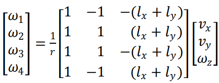
Figure 9: Forward Kinematic Model: this matrix translates a required velocity in 2D and a rotation around Z axis (omega z) into angular velocities at each wheel of the robot. lx is half the distance between the front wheels, ly is half the distance between the fron and rear wheels, and r is the radius of the wheel. Source: Taheri et al (2015)

2.5 Control

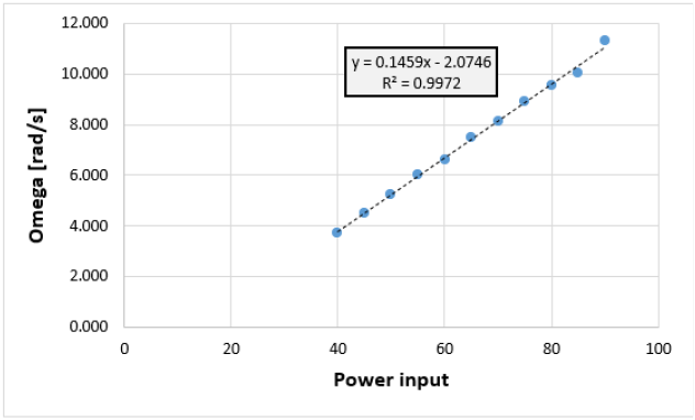
This module is responsible for translating the angular velocities \((\omega_1, \omega_2, \omega_3, \omega_4)\) required by the Short-term Planning module into motor commands to achieve those velocities. Sometimes this task is also called “calibration”. To do this, I sampled multiple straight trajectories of the robot given different motor commands (which I refer to “power”, they could be anywhere from -5000 to 5000). With this experiment I could get a function relating power to the wheel to angular velocity of the wheel, as shown in Figure 10.

Figure 10: This graph shows the relation between power (the motor command interface provided by the robot) and the actual angular velocity achieved. Two things to notice: first, this calibration only works for the surface it was measured because of different friction coefficients, and second, notice that below a power input of 40 the robot won't move because of this friction.

3 Results

3.1 Robot trajectory

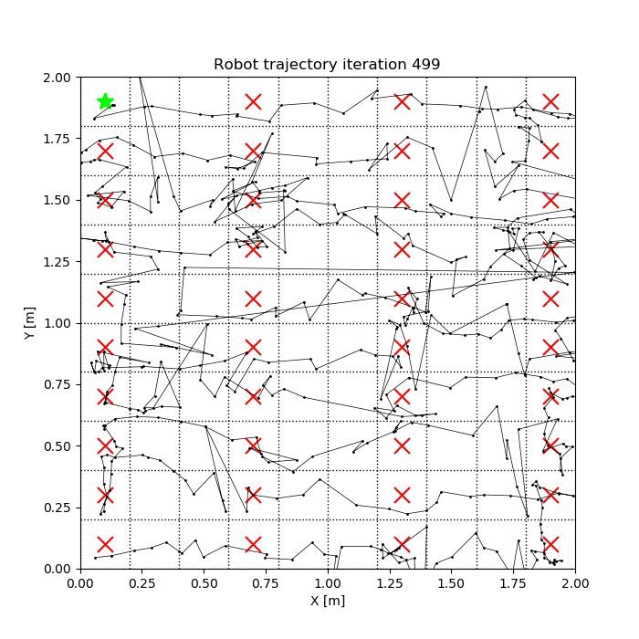
In Figure 11 we show the trajectory estimated by the robot perception stack throught its journey. The video associated to this experiment can be seen in this link: https://youtu.be/yTnWUw7eKxI.

Figure 11: This plot shows the beginning of the trajectory (estimated by the robot) in the green star up to the point near (0,0). The system is very noisy because of the quality of the sensors is not good, nonetheless, the robot managed to cover the area in a reasonable time.

3.2 Performance guarantee

In this section we explain a simplified approach to provide a performance guarantee considering only a single dimension. The question we are trying to answer here is: what is the expected coverage percentage of our robot in a 1D grid cell, considering that the localization error follows a probability distribution and that the robot is considered to cover that cell when it is at a minimum threshold distance? Figure 12 shows our method.

Figure 12: his diagram shows our simplified approach for estimating the stochastic coverage of a 1D cell. If there was no error noise and a threshold τ = 0, the robot estimate would be the same as the center of the cell (star icon), thus achieving a 100% coverage. But, because of noise, we allow the robot to mark the cell as covered when being within a threshold τ of its center, so in the best case the robot is going to be τ from the real center of the cell. On top of this, we know the localization error follows a probability distribution, so can sample a value from this distribution to get a stochastic estimate of the real position of the robot. That would give us the real coverage of the robot given by the intersection of the robot interval and the cell interval, which is the red interval.

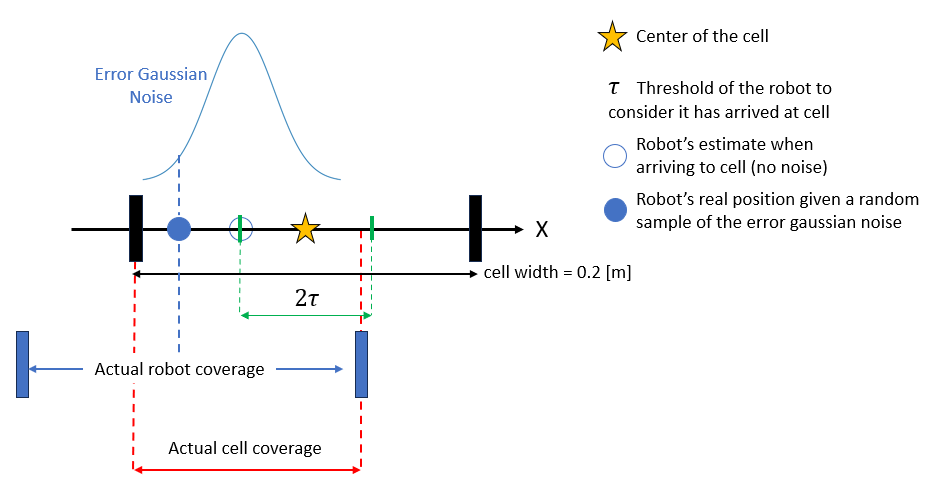
By using Monte Carlo simulation on this stochastic system we can expect on average, that each cell of the grid is going to be covered roughly by 47% on the first pass of the roomba.