Visual Odometry

This is the Visual Odometry Lab from the Self-Driving Cars Specialization from Coursera.

Project repository: https://github.com/fjzs/VisualOdometry

What is Visual Odometry?

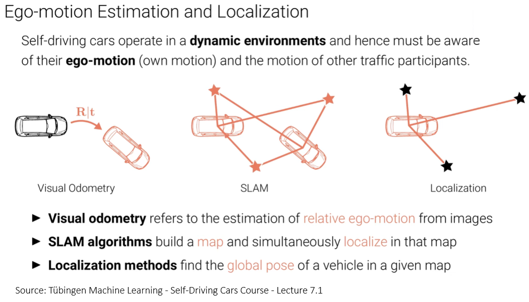
Visual Odometry is the task of estimating the relative ego-motion from images. The output is a rigid body transformation \(R|t\) with 6 degrees of freedom. Because this task yields relative motion estimates (not global position with respect to a map), it is sensitive to error acumulation over time. This is why it is said to be precise locally only.

In this lab we had to estimate the trajectory of a car given:

• \(T\) consecutive RGB images (from CARLA simulator) taken by the car at every time step \(t\in{1,2,...,T}\)
• Depth information for every image (every pixel indicates the length in meters to that point)
• Intrinsic camera parametrs \(K\).

To accomplish this I had to:

1. Extract features from the images
2. Match features
3. Estimate camera motion between a consecutive images

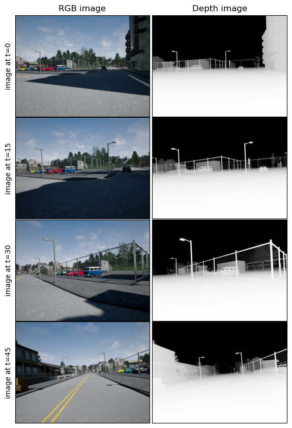
First of all, let’s look at some images to get a notion of the data. In the figure below, you will see the RGB and depth images from the CARLA simulator for time steps [0, 15, 30, 45]. In the depth image, black color represents far locations and white color represents closer locations.

(1) Extracting features

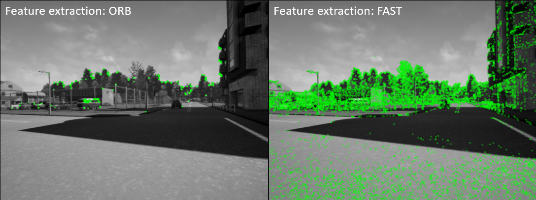
To extract features I tried ORB and FAST methods from OpenCV. Although both methods had hyperparameters that could be tuned, I decided to continue with ORB because I found it to be easy to control. In the picture below you can see the features detected for the first image of the dataset for both methods with default hyperparameters.

(2) Matching features

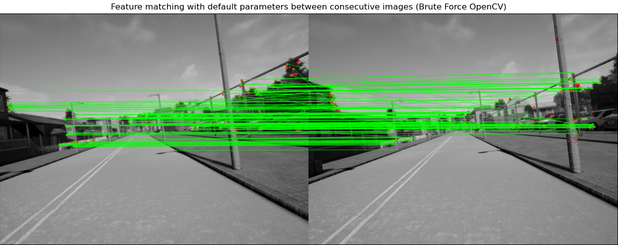
Feature matching can be done in multiple ways, with learning and non-learning algorithms. In this lab I decided to proceed with the simplest approach before trying more complex ones. In particular, I used the Brute Force Matcher implementation from OpenCV. In the picture below you can see how this algorithm performs with default parameters. Interesting things to notice:

• The red points are features that the matcher could not match between images
• Most of the matches are correct (horizontal lines, because the camera motion between frames is tiny)
• Some matches are incorrect (diagonal lines)

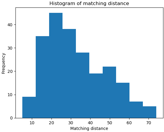
Although we have good features, we can see some incorrect matches (given by diagonal lines) that can introduce problems downstream in the problem. To solve this I decided to use a threshold to avoid matches above a certain value. Of course more complex methods exists (based on deep learning), but we are avoiding those for simplicity to get the pipeline running. The image below shows an histogram of the matching distance so as to have an idea of a good threshold value. I decided to cut every match with a distance greater than 40 to minimize the impact of false positives.

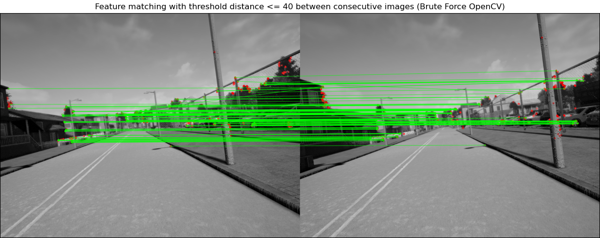
After using the threshold of 40 the matches look slightly better (there are less diagonal lines), and the cost we had to pay was to obtain less matches. You can see the result in the following figure.

(3) Estimating camera motion between consecutive images

Now that we have consecutive frames with matched features we can estimate the camera motion between those frames. To do this we can:

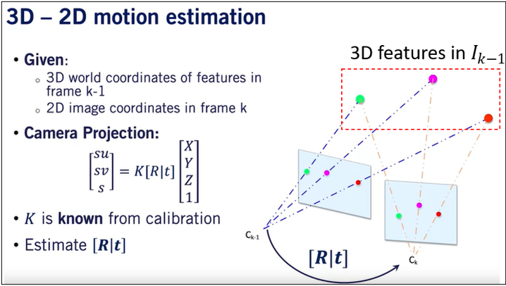
1. Use the Perspective-n-Point (PnP) algorithm, which uses the depth information also.
2. Use the Essential Matrix Decomposition, which does not use the depth information.

In both methods we can incorporate RANSAC algorithm to handle outliers.

I decided to proceed with PnP algorithm, which is offered in OpenCV with a RANSAC option as well. It needs at least 3 points to solve the optimization problem wich would return 4 ambiguous solutions. If four or more points are provided, then the algorithm returns a single solution. Given that we have dozens of matching features, we will always get the unique solution to the problem. The figure below illustrates the optimization problem to solve.

After applying this algorithm, we will retrieve \([R|t]\), now, what does that matrix exactly represents? It represents the transformation needed to go from camera center at time step \(t\) to camera center at time step \(t-1\), which I’ll denote as:

Computing the trajectory of the camera is equivalent to compute the camera position (center and pose) at all timesteps (or frames), expressing them in the coordinate frame of time step \(t=0\). In other words, the trajectory is:

Where \(O_t^k\) represents the position of the origin in image \(t\) in the coordinate frame of camera at time step \(k\).

We know that \(O_0^0=[0,0,0,1]\) because this is the origin of the camera at time step \(t=0\) (using homogeneous coordinates). We also know that:

Given that the PnP algorithm estimated in the first iteration \(T^{1,0}\), we can get obtain the reverse transformation:

Therefore:

How about \(O^0_i\)? with a little of algebra you will arrive to the following expression:

But the PnP algorithm gives \(T^{i,i-1}\) so you take the inverse and replace it in the formula to get every element in the trajectory. Remember that \(O_i^i=[0,0,0,1]\) because we are using homogeneous coordinates.

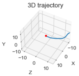
The 3D plot of this trajectory looks like the following figure (and it has a 98% accuracy with respect to the ground truth):

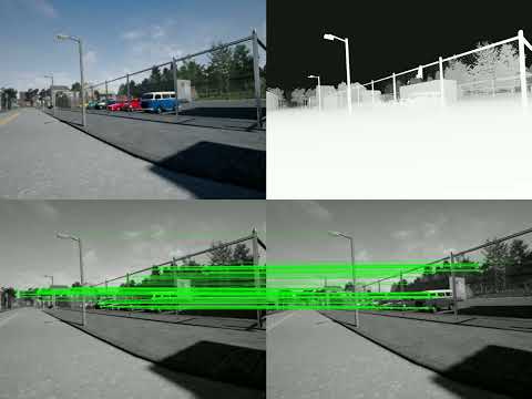
Finally, a YouTube video showing the RGB images, depth images and matching features is linked in the next figure (click on it):